1 符号注解
| 符号 | 解释 |
|---|---|
| \(K\) | 词汇表的大小 |
| \(T\) | 句子的长度 |
| \(H\) | 隐藏层单元数 |
| \(\mathbb{x}={x_1, x_2,...,x_T}\) | 句子的单词序列 |
| \(x_t\in\mathbb{R}^{K\times 1}\) | t时刻RNN的输入,为one-hot vector,1表示一个单词的出现,0表示不出现 |
| \(x\in \mathbb{R}^{T \times K}\) | 一个完整的句子, 句子的长度T |
| \(\hat{y}_t\in\mathbb{R}^{K\times 1}\) | t时刻softmax层的输出, 估计每个词出现的概率, 有时用\(o_t\) |
| \(y_t\in\mathbb{R}^{K\times 1}\) | t时刻的label, 真实每个词出现的概率, one-hot vector. |
| \(E_t\) | 第t个时刻(第t个word)的损失函数,定义为交叉熵误差\(E_t=−y_t^Tlog(\hat{y}_t)\) |
| \(E\) | 一个句子的损失函数,由各个时刻(即每个word)的损失函数组成,\(E=\sum\limits_t^T E_t\). |
| \(s_t\in\mathbb{R}^{H\times 1}\) | t个时刻RNN隐藏层的输入 |
| \(h_t\in\mathbb{R}^{H\times 1}\) | t个时刻RNN隐藏层的输出 |
| \(z_t\in\mathbb{R}^{K\times 1}\) | 输出层的汇集输入 (空间映射:H到K) |
| \(r_t=\hat{y}_t−y_t\) | 残差向量 |
| \(W\in\mathbb{R}^{H\times K}\) | 从输入层到隐藏层的权值 |
| \(U\in\mathbb{R}^{H\times H}\) | 隐藏层上一个时刻到当前时刻的权值 |
| \(V\in\mathbb{R}^{K\times H}\) | 隐藏层到输出层的权值 |
函数关系:
\[ \left\{ \begin{align*} s_t &= Uh_{t-1} + Wx_t \\ h_t &= tanh(s_t) \\ z_t &= Vh_t \\ \hat{y}_t &= softmax(z_t) \\ E_t &= -y_t^Tlog\hat{y}_t \\ \end{align*} \right. \]
由于\(x_t, y_t\)都是one-hot vector, 可以得出以下几点:
\(Wx_t\) 如果是输入的是第j个词(对应j值1, 其余为0), 计算结果简化为将\(W\)的第j列取出.
当前时刻交叉熵\(E_t=-y_t^Tlog(\hat{y}_t) = -log(\hat{y}_t,j\), 即如果t时出现的是第j个词, 只需要看 \(\hat{y}_t\)的第j个分量.
2 RNN(BPTT)
2.1 隐马尔可夫模型
Hidden Markov Model(HMM)
dummy 马尔科夫链的核心是说, 在给定当前知识或信息的情况下, 观察对象的过去的历史状态, 对于将来的预测来说预测是无关 的. 也可以说, 在观察一个系统变化的时候, 它下一个状态(n+1)如何的概率只需观察和统计当前状态(n).
隐马尔科夫链是个双重随机过程, 不仅状态转移之间是个随机过程, 状态和输出之间也是个随机过程.

状态的改变是使用虚线表示\(X_1\)到\(X_T\) (隐含状态链), 我们没法直接观察到, 而我们能够直接看到的是状态改变时带 来的观察值的变化\(O_1\)到\(O_T\) (可见状态链). 可见状态之间没有直接的转换概率, 隐含状态和可见状态之间存在一个 概率叫做输出概率
训练模型:
通过输入\(X_i\)和\(O_i\)两个序列, 经过统计学模型训练, 最后得到两个矩阵, 一个是\(X\)之间的隐含状态转移关系的矩阵, 一个是\(X\)到\(O\)之间的输出概率矩阵.
RNN好的地方是它可以记住前面一段时间的输入信息,不好的地方是它只能记住某段时间的输入信息,虽然理论上RNN可以 处理长时间的信息,但是实际上它却不能很好的学习这些信息.对于长时间的输入信息它无能为力.
2.2 BPTT
Backpropagation Through Time(时序反向传播算法):
The parameters are shared by all times in the rnn network, the gradient at each output depends not only the current time steps but also the previous time steps. For example, in order to calculate the gradient at \(t=4\), we would need to backpropagate 3 steps and sum up the gradients.

Formulas:
\(x_t\): one-hot vector, t时刻的输入.
\(s_t\): hidden state, t时候的隐藏状态, 通过前一个隐藏状态和当前输入计算出来的, \(s_t = f(Ux_t + Ws_{t-1})\), f可以是tanh或relu.
\(o_t\): output, \(o_t = softmax(Vs_t)\)
注意, 有的地方还加了一个非线性变换:
\(h_t\): hidden output, \(h_t = tanh(s_t)\)
\(z_t\): output, \(z_t = Vh_t = V tanh(s_t)\)
\(\hat{y}_t = softmax(z_t) = softmax(Vtanh(s_t))\)
模型里是蕴含着这样的逻辑的, 那就是前一次输入的向量\(x_{t-1}\)所产生的结果对于本次输出的结果是有一定的影响的, 甚至更远期的\(x_{t-2}, x_{t-3} ··· ···\)都"潜移默化"地在影响本次输出的结果.
2.2.1 思考
- 为什么隐藏层的输出需要\(V\),即\(\hat{y}_t = softmax(Vz_t)\), 不能直接\(\hat{y}_t = softmax(h_t)\) ?
从变量的类型分析, \(\hat{y}_t \in \mathbb{R}^{K\times 1}, h_t \in \mathbb{R}^{H\times 1}, V \in \mathbb{R}^{K\times H}\), \(V\)矩阵可以把H空间映射到K空间.
- \(U\), \(V\), \(W\)分别有什么意义?
RNN神经网络和传统的神经网络一样由
输入层,隐藏层,输出层组成, 不同的是RNN网络中超参数是共享的, \(W\)将输入层的词向量映射到隐藏层的空间中, \(U\)是自身状态的映射, 结合上下文进行记忆的取舍, \(W\)结合\(U\)形成当前时刻的隐藏层的知识状态, \(V\)是隐藏层到输出层的映射. \(U\)为输入权重, \(W\)为递归权重; \(V\)为输出权重
There are a few things to note here:
dummy
You can think of the hidden state s_t as the memory of the network. s_t captures information about what happened in all the previous time steps. The output at step o_t is calculated solely based on the memory at time t. As briefly mentioned above, it's a bit more complicated in practice because s_t typically can't capture information from too many time steps ago.
Unlike a traditional deep neural network, which uses different parameters at each layer, a RNN shares the same parameters (U, V, W above) across all steps. This reflects the fact that we are performing the same task at each step, just with different inputs. This greatly reduces the total number of parameters we need to learn.
The above diagram has outputs at each time step, but depending on the task this may not be necessary. For example, when predicting the sentiment of a sentence we may only care about the final output, not the sentiment after each word. Similarly, we may not need inputs at each time step. The main feature of an RNN is its hidden state, which captures some information about a sequence.
2.2.2 梯度
完整图:
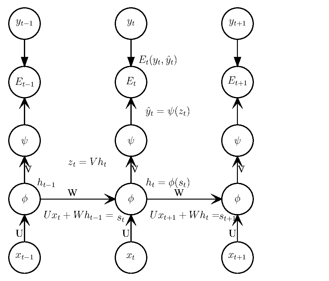
从上图可以看到, 梯度不仅从空间结构上传播(纵向), 而且从时间结构上传播(横向), 这也是BPTT名字的由来.
if:
\(\phi\) is \(tanh()\)
\(\psi\) is \(softmax()\)
损失函数使用CEE(cross entropy loss), 总误差(所有输出节点的误差总和):
\[ \begin{align*} E_t(y_t, \hat{y}_t) &= -\dfrac{1}{n}y_tlog\hat{y}_t \\ E(y, \hat{y}) &= \sum_t E_t(y_t, \hat{y}_t) \\ &= - \sum_t y_tlog\hat{y}_t \end{align*} \]
then:
\[ \begin{align*} \dfrac{\partial E_t}{\partial z_t} &= \dfrac{\partial E_t}{\partial \hat{y}_t} \psi'(z_t) \\ &= \hat{y}_t - y_t \qquad \text{ if } \psi \text { is softmax() } \tag{1} \end{align*} \]
很多公式某些地方没考虑矩阵或向量不同维度相乘的情况, 不是很严谨(严格说是错误的), 仅供参考.
- 对\(V\)梯度
\[ \begin{align*} \dfrac{\partial E_t}{\partial V} &= \dfrac{\partial E_t}{\partial z_t} \dfrac{\partial z_t}{\partial V} \\ &= \dfrac{\partial E_t}{\partial \hat{y}_t} \psi'(z_t) \otimes h_t \\ &= (\hat{y} - y_t) {h_t}^T \tag{2} \\ \end{align*} \]
\[ \dfrac{\partial E}{\partial V} = \sum_{k=0}{t} (\hat{y}_k - y_k) \otimes h_k \]
只和当前状态的输出有关.
- 对\(U\)求梯度
\[ \begin{align*} \dfrac{\partial E_t}{\partial U} &= \dfrac{\partial E_t}{\partial z_t} \dfrac{\partial z_t}{\partial h_t} \phi'(s_t) \dfrac{\partial s_t}{\partial U} \dfrac{\partial s_t}{\partial h_{t-1}} \phi'(s_{t-1}) \dfrac{\partial s_{t-1}}{\partial U}\cdots \\ &= \dfrac{\partial E_t}{\partial z_t} V^T \phi'(s_t) \dfrac{\partial s_t}{\partial U} W^T \phi'(s_{t-1}) \dfrac{\partial s_{t-1}}{\partial U}\cdots \\ &= \sum_{k=1}^{t} \dfrac{\partial E_t}{\partial z_t}\dfrac{\partial z_t}{\partial h_t} \dfrac{\partial h_t}{\partial h_k} \dfrac{\partial h_k}{\partial s_k} \dfrac{\partial s_k}{\partial U} \\ &= \sum_{k=1}^{t} \dfrac{\partial E_t}{\partial h_k} \dfrac{\partial h_k}{\partial s_k} {x_k}^T \tag {3} \end{align*} \]
由于\(s_t\)的上一个状态输出\(h_{t-1}\)依然含有\(U\)的分量, 形式变为:
- 对\(W\)求梯度
\[ \begin{align*} \dfrac{\partial E_t}{\partial W} &= \dfrac{\partial E_t}{\partial z_t} \dfrac{\partial z_t}{\partial h_t} \phi'(s_t) \dfrac{\partial s_t}{\partial W} \dfrac{\partial s_t}{\partial h_{t-1}} \phi'(s_{t-1}) \dfrac{\partial s_{t-1}}{\partial W}\cdots \\ &= \dfrac{\partial E_t}{\partial z_t} V^T \phi'(s_t) \dfrac{\partial s_t}{\partial W} W^T \phi'(s_{t-1}) \dfrac{\partial s_{t-1}}{\partial W}\cdots \\ &= \sum_{k=1}^{t} \dfrac{\partial E_t}{\partial z_t}\dfrac{\partial z_t}{\partial h_t} \dfrac{\partial h_t}{\partial h_k} \dfrac{\partial h_k}{\partial s_k} \dfrac{\partial s_k}{\partial W} \\ &= \sum_{k=1}^{t} \dfrac{\partial E_t}{\partial h_k} \dfrac{\partial h_k}{\partial s_k} {h_{k-1}}^T \tag {4} \end{align*} \]
另\(h_0\)全0向量.
2.2.3 计算例子
形式和上面的有些不同, 隐藏层输入和隐藏层输出合成一个\(s_t = tanh(Ux_t + Ws_{t-1})\).

let:
- formulas
\[ \begin{aligned} & s_0 = tanh(U x_0 + W s_{-1}) \\ & z_0 = V s_0 \\ & o_0 \triangleq \hat{y}_{0} = sigmoid(z_0) \\\\ & s_1 = tanh(U x_1 + W s_0) \\ & z_1 = V s_1 \\ & o_1 \triangleq \hat{y}_{1} = sigmoid(z_1) \\\\ & s_2 = tanh(U x_2 + W s_1) \\ & z_2 = V s_2 \\ & o_2 \triangleq \hat{y}_{2} = sigmoid(z_2) \\\\ & s_3 = tanh(U x_3 + W s_2) \\ & z_3 = V s_3 \\ & o_3 \triangleq \hat{y}_{3} = sigmoid(z_3) \\ \end{aligned} \]
- loss
\[ \begin{aligned} L(y, o) = - \frac{1}{N}\sum_{n \in N}y_n \log o_n \end{aligned} \]
- partial derivative
if: \(d_t \triangleq \dfrac{\partial E_t}{\partial s_t}\) then:
\[ \begin{aligned} & d_3 \triangleq \big(\hat{y}_3 - y_3 \big) \cdot V \cdot \big(1 - s_3 ^ 2 \big) \\ & d_2 \triangleq d_3 \cdot W \cdot \big(1 - s_2 ^ 2 \big) \\ & d_1 \triangleq d_2 \cdot W \cdot \big(1 - s_1 ^ 2 \big) \\ & d_0 \triangleq d_1 \cdot W \cdot \big(1 - s_0 ^ 2 \big) \\ \end{aligned} \]
so calculate dLdV, dLdU, dLdW:
- \(\frac{\partial{L}}{\partial{V}}\)
\[ \begin{aligned} \frac{\partial{E_3}}{\partial{V}} &= \frac{\partial{E_3}}{\partial{\hat{y}_3}} \frac{\partial{\hat{y}_3}}{\partial{z_3}} \frac{\partial{z_3}}{\partial{V}} \\ &= (\hat{y}_{3} - y_3) s_3 \end{aligned} \]
- \(\frac{\partial{L}}{\partial{U}}\)
\[ \begin{aligned} \frac{\partial{s_0}}{\partial{U}} &= \big(1 - s_0 ^ 2 \big) \left(x_0 + \frac{\partial{s_{-1}}}{\partial{U}} \right) \\ &= \big(1 - s_0 ^ 2 \big) \cdot x_0 \\\\ \frac{\partial{s_1}}{\partial{U}} &= \big(1 - s_1 ^ 2 \big) \left(x_1 + W \cdot \frac{\partial{s_{0}}}{\partial{U}} \right) \\ &= \big(1 - s_1 ^ 2 \big) \big(x_1 + W \cdot \big(1 - s_0 ^ 2 \big) \cdot x_0 \big) \\\\ \frac{\partial{s_2}}{\partial{U}} &= \big(1 - s_2 ^ 2 \big) \left(x_2 + W \cdot \frac{\partial{s_{1}}}{\partial{U}} \right) \\ &= \big(1 - s_2 ^ 2 \big) \Big(x_2 + W \cdot \big(1 - s_1 ^ 2 \big) \big(x_1 + W \cdot \big(1 - s_0 ^ 2 \big) \cdot x_0 \big) \Big)\\\\ \frac{\partial{s_3}}{\partial{U}} &= \big(1 - s_3 ^ 2 \big) \left(x_3 + W \cdot \frac{\partial{s_{2}}}{\partial{U}} \right) \\ &= \big(1 - s_3 ^ 2 \big) \\ & \bigg(x_3 + W \cdot \big(1 - s_2 ^ 2 \big) \Big(x_2 + W \cdot \big(1 - s_1 ^ 2 \big) \big(x_1 + W \cdot \big(1 - s_0 ^ 2 \big) \cdot x_0 \big) \Big) \bigg)\\\\ \end{aligned} \]
\[ \begin{aligned} \frac{\partial{E_3}}{\partial{U}} &= \frac{\partial{E_3}}{\partial{\hat{y}_3}} \frac{\partial{\hat{y}_3}}{\partial{z_3}} \frac{\partial{z_3}}{\partial{s_3}} \frac{\partial{s_3}}{\partial{U}} \\ &= \left(\frac{\partial{E_3}}{\partial{\hat{y}_3}} \frac{\partial{\hat{y}_3}}{\partial{z_3}} \right) \cdot \frac{\partial{z_3}}{\partial{s_3}} \cdot \frac{\partial{s_3}}{\partial{U}} \\ &= \big(\hat{y}_3 - y_3 \big) \cdot V \cdot \frac{\partial{s_3}}{\partial{U}} \\ &= \big(\hat{y}_3 - y_3 \big) \cdot V \cdot \big(1 - s_3 ^ 2 \big) \bigg(x_3 + W \cdot \big(1 - s_2 ^ 2 \big) \Big(x_2 + W \cdot \big(1 - s_1 ^ 2 \big) \big(x_1 + W \cdot \big(1 - s_0 ^ 2 \big) \cdot x_0 \big) \Big) \bigg)\\ & \triangleq d_3 \big[x_3 + W \cdot \big(1 - s_2 ^ 2 \big) \Big(x_2 + W \cdot \big(1 - s_1 ^ 2 \big) \big(x_1 + W \cdot \big(1 - s_0 ^ 2 \big) \cdot x_0 \big) \Big) \big]\\ &= d_3 x_3 + d_3 W \cdot \big(1 - s_2 ^ 2 \big) \Big(x_2 + W \cdot \big(1 - s_1 ^ 2 \big) \big(x_1 + W \cdot \big(1 - s_0 ^ 2 \big) \cdot x_0 \big) \Big) \\ & \triangleq d_3 x_3 + d_2 \Big(x_2 + W \cdot \big(1 - s_1 ^ 2 \big) \big(x_1 + W \cdot \big(1 - s_0 ^ 2 \big) \cdot x_0 \big)\Big) \\ &= d_3 x_3 + d_2 x_2 + d_2 W \cdot \big(1 - s_1 ^ 2 \big) \big(x_1 + W \cdot \big(1 - s_0 ^ 2 \big) \cdot x_0 \big) \\ & \triangleq d_3 x_3 + d_2 x_2 + d_1 \big(x_1 + W \cdot \big(1 - s_0 ^ 2 \big) \cdot x_0 \big) \\ &= d_3 x_3 + d_2 x_2 + d_1 x_1 + d_1 W \cdot \big(1 - s_0 ^ 2 \big) \cdot x_0 \\ & \triangleq d_3 x_3 + d_2 x_2 + d_1 x_1 + d_0 \cdot x_0 \\ \end{aligned} \]
- \(\frac{\partial{L}}{\partial{W}}\)
\[ \begin{aligned} \frac{\partial{s_0}}{\partial{W}} &= \big(1 - s_0 ^ 2 \big) \left(s_{-1} + \frac{\partial{s_{-1}}}{\partial{W}} \right) \\ &= \big(1 - s_0 ^ 2 \big) \cdot s_{-1} \\\\ \frac{\partial{s_1}}{\partial{W}} &= \big(1 - s_1 ^ 2 \big) \left(s_0 + W \cdot \frac{\partial{s_{0}}}{\partial{W}} \right) \\ &= \big(1 - s_1 ^ 2 \big) \big(s_0 + W \cdot \big(1 - s_0 ^ 2 \big) \cdot s_{-1} \big) \\\\ \frac{\partial{s_2}}{\partial{W}} &= \big(1 - s_2 ^ 2 \big) \left(s_1 + W \cdot \frac{\partial{s_{1}}}{\partial{W}} \right) \\ &= \big(1 - s_2 ^ 2 \big) \Big(s_1 + W \cdot \big(1 - s_1 ^ 2 \big) \big(s_0 + W \cdot \big(1 - s_0 ^ 2 \big) \cdot s_{-1} \big) \Big)\\\\ \frac{\partial{s_3}}{\partial{W}} &= \big(1 - s_3 ^ 2 \big) \left(s_2 + W \cdot \frac{\partial{s_{2}}}{\partial{W}} \right) \\ &= \big(1 - s_3 ^ 2 \big) \bigg(s_2 + W \cdot \big(1 - s_2 ^ 2 \big) \Big(s_1 + W \cdot \big(1 - s_1 ^ 2 \big) \big(s_0 + W \cdot \big(1 - s_0 ^ 2 \big) \cdot s_{-1} \big) \Big) \bigg)\\\\ \end{aligned} \]
\[ \begin{aligned} \frac{\partial{E_3}}{\partial{W}} &= \frac{\partial{E_3}}{\partial{\hat{y}_3}} \frac{\partial{\hat{y}_3}}{\partial{z_3}} \frac{\partial{z_3}}{\partial{s_3}} \frac{\partial{s_3}}{\partial{W}} \\ &= \left(\frac{\partial{E_3}}{\partial{\hat{y}_3}} \frac{\partial{\hat{y}_3}}{\partial{z_3}} \right) \cdot \frac{\partial{z_3}}{\partial{s_3}} \cdot \frac{\partial{s_3}}{\partial{W}} \\ &= \big(\hat{y}_3 - y_3 \big) \cdot V \cdot \frac{\partial{s_3}}{\partial{W}} \\ &= \big(\hat{y}_3 - y_3 \big) \cdot V \cdot \big(1 - s_3 ^ 2 \big) \bigg(s_2 + W \cdot \big(1 - s_2 ^ 2 \big) \Big(s_1 + W \cdot \big(1 - s_1 ^ 2 \big) \big(s_0 + W \cdot \big(1 - s_0 ^ 2 \big) \cdot s_{-1} \big) \Big) \bigg)\\ & \triangleq d_3 \bigg(s_2 + W \cdot \big(1 - s_2 ^ 2 \big) \Big(s_1 + W \cdot \big(1 - s_1 ^ 2 \big) \big(s_0 + W \cdot \big(1 - s_0 ^ 2 \big) \cdot s_{-1} \big) \Big) \bigg) \\ &= d_3 s_2 + d_3 W \cdot \big(1 - s_2 ^ 2 \big) \Big(s_1 + W \cdot \big(1 - s_1 ^ 2 \big) \big(s_0 + W \cdot \big(1 - s_0 ^ 2 \big) \cdot s_{-1} \big) \Big) \\ & \triangleq d_3 s_2 + d_2 \Big(s_1 + W \cdot \big(1 - s_1 ^ 2 \big) \big(s_0 + W \cdot \big(1 - s_0 ^ 2 \big) \cdot s_{-1} \big) \Big) \\ &= d_3 s_2 + d_2 s_1 + d_2 W \cdot \big(1 - s_1 ^ 2 \big) \big(s_0 + W \cdot \big(1 - s_0 ^ 2 \big) \cdot s_{-1} \big) \\ & \triangleq d_3 s_2 + d_2 s_1 + d_1 \big(s_0 + W \cdot \big(1 - s_0 ^ 2 \big) \cdot s_{-1} \big) \\ &= d_3 s_2 + d_2 s_1 + d_1 s_0 + d_1 W \cdot \big(1 - s_0 ^ 2 \big) \cdot s_{-1} \\ & \triangleq d_3 s_2 + d_2 s_1 + d_1 s_0 + d_0 \cdot s_{-1} \\ \end{aligned} \]
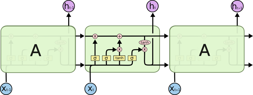
3 LSTM
3.1 长期依赖
LSTM 解决避免长时期依赖(long-term dependency)的问题
3.2 梯度消失
LSTM 在某种程度上可以克服梯度消失问题.
图片来自1
3.3 与标准RNN对比
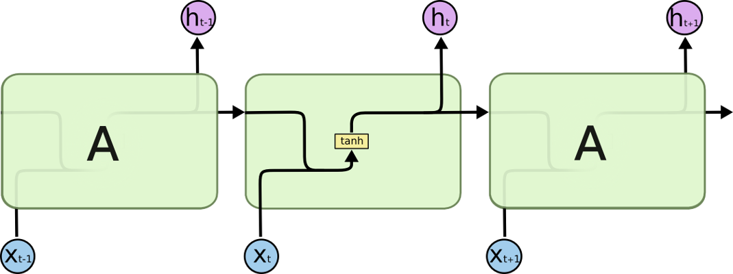
VS
非常详细的介绍请点击这里
4 应用场景
4.1 语音识别
4.2 语言翻译
4.3 股票预测
4.4 图像识别(图里的内容)
5 其他
5.1 关键字
神经注意力模块(Attention) = 向前预测单元 + 后向回顾单元
6 References
- Understanding LSTM Networks
- 译 Understanding LSTM Networks
- Pytorch RNN
- 如何深度理解RNN?——看图就好!
- Attention Is All You Need
- recurrent-neural-networks-tutorial-part-1-introduction-to-rnns
- recurrent-neural-networks-tutorial-part-3-backpropagation-through-time-and-vanishing-gradients
- BTPP推导1
- BTPP推导2
- deriving-back-propagation-on-simple-rnn-lstm
- RNN-BPTT
- build-recurrent-neural-network-from-scratch
https://baijiahao.baidu.com/s?id=1612358810937334377&wfr=spider&for=p↩